R and tidyverse for publicly available Nordic data on medication utilization
Elena Dudukina
2020-10-10
1 / 42
National Registries
- Denmark and other Nordic countries have built a system based on societal trust and enabled state-covered universal healthcare
- Large administrative registries with data on hospital visits and prescription drug utilization
- Amazing possibilities for a high quality registry-based research
- Many registries can be accessible to a public via aggregated datasets
- The National Prescription Registry (since 1995)
- Drug utilization trends and between countries comparisons
2 / 42
Loading libraries and finding autumn palette
library(tidyverse)library(magrittr)library(colorfindr)library(ggrepel)autumn_colors <- get_colors("https://images2.minutemediacdn.com/image/upload/c_crop,h_1349,w_2400,x_0,y_125/f_auto,q_auto,w_1100/v1569260079/shape/mentalfloss/gettyimages-1053614486_1.jpg") %>% make_palette(n = 15)
3 / 42
Prepare to load data on 
link_list_dk <- list( "1996_atc_code_data.txt" = "https://medstat.dk/da/download/file/MTk5Nl9hdGNfY29kZV9kYXRhLnR4dA==", "1997_atc_code_data.txt" = "https://medstat.dk/da/download/file/MTk5N19hdGNfY29kZV9kYXRhLnR4dA==", "1998_atc_code_data.txt" = "https://medstat.dk/da/download/file/MTk5OF9hdGNfY29kZV9kYXRhLnR4dA==", "atc_code_text.txt" = "https://medstat.dk/da/download/file/YXRjX2NvZGVfdGV4dC50eHQ=", "atc_groups.txt" = "https://medstat.dk/da/download/file/YXRjX2dyb3Vwcy50eHQ=", "population_data.txt" = "https://medstat.dk/da/download/file/cG9wdWxhdGlvbl9kYXRhLnR4dA==")The actual number of files is 23, from 1996 until 2019 and 3 additional files with meta-data, e.g., variables' labels
4 / 42
Data on population sizes of each age group and sex
# age structure data# parse with column type characterage_structure <- read_delim(link_list_dk[["population_data.txt"]], delim = ";", col_names = c(paste0("V", c(1:7))), col_types = cols(V1 = col_character(), V2 = col_character(), V3 = col_character(), V4 = col_character(), V5 = col_character(), V6 = col_character(), V7 = col_character())) %>% # rename and keep columns select(year = V1, region_text = V2, region = V3, gender = V4, age = V5, denominator_per_year = V6) %>% # human-reading friendly label on sex categories mutate( gender_text = case_when( gender == "0" ~ "both sexes", gender == "1" ~ "men", gender == "2" ~ "women", T ~ as.character(gender) ) ) %>% # make numeric variables mutate_at(vars(year, age, denominator_per_year), as.numeric) %>% # keep only data for the age categories I will work with, only on women, and for the whole Denmark filter(age %in% 15:84, gender == "2", region == "0") %>% arrange(year, age, region, gender)5 / 42
Data structure
age_structure %>% slice(1:10)## # A tibble: 10 x 7## year region_text region gender age denominator_per_year gender_text## <dbl> <chr> <chr> <chr> <dbl> <dbl> <chr> ## 1 1996 DK 0 2 15 29092 women ## 2 1996 DK 0 2 16 29961 women ## 3 1996 DK 0 2 17 31344 women ## 4 1996 DK 0 2 18 31419 women ## 5 1996 DK 0 2 19 32494 women ## 6 1996 DK 0 2 20 36363 women ## 7 1996 DK 0 2 21 36366 women ## 8 1996 DK 0 2 22 36498 women ## 9 1996 DK 0 2 23 38452 women ## 10 1996 DK 0 2 24 37873 women6 / 42
Prepare labels for the drugs in English
eng_drug <- read_delim(link_list_dk[["atc_groups.txt"]], delim = ";", col_names = c(paste0("V", c(1:6))), col_types = cols(V1 = col_character(), V2 = col_character(), V3 = col_character(), V4 = col_character(), V5 = col_character(), V6 = col_character())) %>% # keep drug classes labels in English filter(V5 == "1") %>% select(ATC = V1, drug = V2, unit_dk = V4)7 / 42
Check drugs' labels
eng_drug %>% slice(1:10)## # A tibble: 10 x 3## ATC drug unit_dk ## <chr> <chr> <chr> ## 1 A Alimentary tract and metabolism No common unit for volume## 2 A01 Stomatological preparations No common unit for volume## 3 A01A Stomatological preparations No common unit for volume## 4 A01AA Caries prophylactic agents Packages ## 5 A01AA01 Sodium fluoride Packages ## 6 A01AB Antiinfectives for local oral treatment No common unit for volume## 7 A01AB02 Hydrogenperoxide <NA> ## 8 A01AB03 Chlorhexidine DDD ## 9 A01AB04 Amphotericin DDD ## 10 A01AB09 Miconazole DDD8 / 42
Drugs of interest
Medications used in Denmark for either migraine episode relief or migraine prophylaxis:
I use regular expresions (regex) to capture the drugs codes of interest
$ at the end of the regular expression tells to my search strategy what is the last character of the string
Example:
codes <- c("N02CC", "N02C", "N02CC01", "N02CC01", "N02CC02", "N02CC")only_want_N02C_regex <- "N02C$"only_want_N02CC_regex <- "N02CC$"want_any_N02C_regex <- "N02CC"str_extract(string = codes, pattern = only_want_N02C_regex)## [1] NA "N02C" NA NA NA NAstr_extract(string = codes, pattern = only_want_N02CC_regex)## [1] "N02CC" NA NA NA NA "N02CC"str_extract(string = codes, pattern = want_any_N02C_regex)## [1] "N02CC" NA "N02CC" "N02CC" "N02CC" "N02CC"9 / 42
Specify all the drug codes I need
regex_triptans <- "N02CC$"regex_ergots <- "N02CA$"regex_nsaid <- "M01A$"regex_naproxen <- "M01AE02$"regex_erenumab <- "N02CX07$|N02CD01$"regex_galcanezumab <- "N02CX08$|N02CD02$"regex_fremanezumab <- "N02CD03$"regex_paracet <- "N02BE01$"regex_salyc_acid_caff <- "N02BA51$"regex_metoclopramide <- "A03FA01$"regex_domperidone <- "A03FA03$"regex_metoprolol <- "C07AB02$"regex_propanolol <- "C07AA05$"regex_tolfenamic <- "M01AG02$"regex_topiramate <- "N03AX11$"regex_valproate <- "N03AG01$"regex_flunarizine <- "N07CA03$"regex_amitriptyline <- "N06AA09$"regex_gabapentin <- "N03AX12$"regex_pizotifen <- "N02CX01$"regex_lisinopril <- "C09AA03$"regex_candesartan <- "C09CA06$"regex_riboflavin <- "A11HA04$"regex_botulinum <- "M03AX01$"10 / 42
Load main data
# ATC dataatc_data <- map(atc_code_data_list, ~read_delim(file = .x, delim = ";", trim_ws = T, col_names = c(paste0("V", c(1:14))), col_types = cols(V1 = col_character(), V2 = col_character(), V3 = col_character(), V4 = col_character(), V5 = col_character(),V6 = col_character(), V7 = col_character(), V8 = col_character(), V9 = col_character(), V10 = col_character(), V11 = col_character(), V12 = col_character(), V13 = col_character(), V14 = col_character()))) %>% # bind data from all years bind_rows()11 / 42
Typical data structure
of a medication utilization file from the source
atc_data %>% slice(1:10)## # A tibble: 10 x 14## V1 V2 V3 V4 V5 V6 V7 V8 V9 V10 V11 V12 V13 ## <chr> <chr> <chr> <chr> <chr> <chr> <chr> <chr> <chr> <chr> <chr> <chr> <chr>## 1 A 1996 0 0 A A <NA> <NA> 9854… 4943… <NA> <NA> <NA> ## 2 A01 1996 0 0 A A <NA> <NA> 19180 2776 <NA> <NA> <NA> ## 3 A01A 1996 0 0 A A <NA> <NA> 19180 2776 <NA> <NA> <NA> ## 4 A01AA 1996 0 0 A A <NA> <NA> 1604 0 11 0 <NA> ## 5 A01A… 1996 0 0 A A <NA> <NA> 1604 0 11 0 <NA> ## 6 A01AB 1996 0 0 A A <NA> <NA> 12782 2253 <NA> <NA> <NA> ## 7 A01A… 1996 0 0 A A <NA> <NA> 3157 0 36404 19 <NA> ## 8 A01A… 1996 0 0 A A <NA> <NA> 1689 1 1271 0.7 <NA> ## 9 A01A… 1996 0 0 A A <NA> <NA> 1334 653 121 0.1 <NA> ## 10 A01A… 1996 0 0 A A <NA> <NA> 3547 1599 141 0.1 <NA> ## # … with 1 more variable: V14 <chr>12 / 42
Human-friendly column names
optional, but, hey, easier to follow
atc_data %<>% # rename and keep columns rename( ATC = V1, year = V2, sector = V3, region = V4, gender = V5, age = V6, number_of_people = V7, patients_per_1000_inhabitants = V8, turnover = V9, regional_grant_paid = V10, quantity_sold_1000_units = V11, quantity_sold_units_per_unit_1000_inhabitants_per_day = V12, percentage_of_sales_in_the_primary_sector = V13 )13 / 42
Sneak peek
atc_data %>% slice(1:10)## # A tibble: 10 x 14## ATC year sector region gender age number_of_people patients_per_10…## <chr> <chr> <chr> <chr> <chr> <chr> <chr> <chr> ## 1 A 1996 0 0 A A <NA> <NA> ## 2 A01 1996 0 0 A A <NA> <NA> ## 3 A01A 1996 0 0 A A <NA> <NA> ## 4 A01AA 1996 0 0 A A <NA> <NA> ## 5 A01A… 1996 0 0 A A <NA> <NA> ## 6 A01AB 1996 0 0 A A <NA> <NA> ## 7 A01A… 1996 0 0 A A <NA> <NA> ## 8 A01A… 1996 0 0 A A <NA> <NA> ## 9 A01A… 1996 0 0 A A <NA> <NA> ## 10 A01A… 1996 0 0 A A <NA> <NA> ## # … with 6 more variables: turnover <chr>, regional_grant_paid <chr>,## # quantity_sold_1000_units <chr>,## # quantity_sold_units_per_unit_1000_inhabitants_per_day <chr>,## # percentage_of_sales_in_the_primary_sector <chr>, V14 <chr>14 / 42
Wrangle data
atc_data %<>% # clean columns names and set-up labels mutate( year = as.numeric(year), region_text = case_when( region == "0" ~ "DK", region == "1" ~ "Region Hovedstaden", region == "2" ~ "Region Midtjylland", region == "3" ~ "Region Nordjylland", region == "4" ~ "Region Sjælland", region == "5" ~ "Region Syddanmark", T ~ NA_character_ ), gender_text = case_when( gender == "0" ~ "both sexes", gender == "1" ~ "men", gender == "2" ~ "women", T ~ as.character(gender) ) ) %>% # reformat all variables, which should be numeric as numeric (not character) mutate_at(vars(turnover, regional_grant_paid, quantity_sold_1000_units, quantity_sold_units_per_unit_1000_inhabitants_per_day, number_of_people, patients_per_1000_inhabitants), as.numeric)15 / 42
Sneak peek
atc_data %>% slice(1:10)## # A tibble: 10 x 16## ATC year sector region gender age number_of_people patients_per_10…## <chr> <dbl> <chr> <chr> <chr> <chr> <dbl> <dbl>## 1 A 1996 0 0 A A NA NA## 2 A01 1996 0 0 A A NA NA## 3 A01A 1996 0 0 A A NA NA## 4 A01AA 1996 0 0 A A NA NA## 5 A01A… 1996 0 0 A A NA NA## 6 A01AB 1996 0 0 A A NA NA## 7 A01A… 1996 0 0 A A NA NA## 8 A01A… 1996 0 0 A A NA NA## 9 A01A… 1996 0 0 A A NA NA## 10 A01A… 1996 0 0 A A NA NA## # … with 8 more variables: turnover <dbl>, regional_grant_paid <dbl>,## # quantity_sold_1000_units <dbl>,## # quantity_sold_units_per_unit_1000_inhabitants_per_day <dbl>,## # percentage_of_sales_in_the_primary_sector <chr>, V14 <chr>,## # region_text <chr>, gender_text <chr>16 / 42
Keep only the needed data
atc_data %<>% select(-V14) %>% filter( # only women gender == "2", # country level data region == "0", # prescription medicine only sector =="0") %>% # only drugs of interest filter(str_detect(ATC, all_migraine_drugs)) %>% # deal with non-numeric age and re-code as numeric mutate( age = parse_integer(age) )17 / 42
Keep only the needed data
atc_data %<>% # ages 15 to 80 years filter(age %in% 15:84) %>% # make categories mutate( age_cat = case_when( age %in% 15:24 ~ "15-24", age %in% 25:34 ~ "25-34", age %in% 35:44 ~ "35-44", age %in% 45:54 ~ "45-54", age %in% 55:64 ~ "55-64", age %in% 65:74 ~ "65-74", age %in% 75:84 ~ "75-84", T ~ NA_character_ ))18 / 42
Sneak peek
atc_data %>% slice(1:10)## # A tibble: 10 x 16## ATC year sector region gender age number_of_people patients_per_10…## <chr> <dbl> <chr> <chr> <chr> <int> <dbl> <dbl>## 1 A03F… 1999 0 0 2 15 144 5.47## 2 A03F… 1999 0 0 2 16 222 8.19## 3 A03F… 1999 0 0 2 17 298 10.8 ## 4 A03F… 1999 0 0 2 18 387 13.1 ## 5 A03F… 1999 0 0 2 19 457 15.1 ## 6 A03F… 1999 0 0 2 20 530 16.7 ## 7 A03F… 1999 0 0 2 21 599 18.6 ## 8 A03F… 1999 0 0 2 22 649 19.2 ## 9 A03F… 1999 0 0 2 23 706 18.8 ## 10 A03F… 1999 0 0 2 24 749 20.2 ## # … with 8 more variables: turnover <dbl>, regional_grant_paid <dbl>,## # quantity_sold_1000_units <dbl>,## # quantity_sold_units_per_unit_1000_inhabitants_per_day <dbl>,## # percentage_of_sales_in_the_primary_sector <chr>, region_text <chr>,## # gender_text <chr>, age_cat <chr>19 / 42
Add meta-data
atc_data %<>% # get age groups labels and other meta-data left_join(age_structure) %>% # get drugs' labels left_join(eng_drug)## Joining, by = c("year", "region", "gender", "age", "region_text", "gender_text")## Joining, by = "ATC"20 / 42
Sneak peek
atc_data %>% select(15:19) %>% slice(1:10)## # A tibble: 10 x 5## gender_text age_cat denominator_per_year drug unit_dk## <chr> <chr> <dbl> <chr> <chr> ## 1 women 15-24 26331 Metoclopramide DDD ## 2 women 15-24 27104 Metoclopramide DDD ## 3 women 15-24 27553 Metoclopramide DDD ## 4 women 15-24 29604 Metoclopramide DDD ## 5 women 15-24 30257 Metoclopramide DDD ## 6 women 15-24 31735 Metoclopramide DDD ## 7 women 15-24 32162 Metoclopramide DDD ## 8 women 15-24 33897 Metoclopramide DDD ## 9 women 15-24 37589 Metoclopramide DDD ## 10 women 15-24 37158 Metoclopramide DDD21 / 42
Compute numerators and denomibators
for the age groups of interest
atc_data %<>% group_by(ATC, year, age_cat) %>% mutate( numerator = sum(number_of_people), denominator = sum(denominator_per_year), patients_per_1000_inhabitants = numerator / denominator * 1000 ) %>% filter(row_number() == 1) %>% ungroup() %>% select(year, ATC, drug, unit_dk, gender, age_cat, patients_per_1000_inhabitants) %>% mutate( country = "Denmark" )22 / 42
Sneak peek
atc_data %>% slice(1:10) %>% kableExtra::kable(format = "html")| year | ATC | drug | unit_dk | gender | age_cat | patients_per_1000_inhabitants | country |
|---|---|---|---|---|---|---|---|
| 1999 | A03FA01 | Metoclopramide | DDD | 2 | 15-24 | 15.1281151 | Denmark |
| 1999 | A03FA01 | Metoclopramide | DDD | 2 | 25-34 | 20.4391764 | Denmark |
| 1999 | A03FA01 | Metoclopramide | DDD | 2 | 35-44 | 18.6600845 | Denmark |
| 1999 | A03FA01 | Metoclopramide | DDD | 2 | 45-54 | 21.8477132 | Denmark |
| 1999 | A03FA01 | Metoclopramide | DDD | 2 | 55-64 | 26.4338008 | Denmark |
| 1999 | A03FA01 | Metoclopramide | DDD | 2 | 65-74 | 33.3200827 | Denmark |
| 1999 | A03FA01 | Metoclopramide | DDD | 2 | 75-84 | 42.6086854 | Denmark |
| 1999 | A03FA03 | Domperidone | DDD | 2 | 15-24 | 0.4148186 | Denmark |
| 1999 | A03FA03 | Domperidone | DDD | 2 | 25-34 | 0.4482942 | Denmark |
| 1999 | A03FA03 | Domperidone | DDD | 2 | 35-44 | 0.5565008 | Denmark |
23 / 42
Check if all medication's utilization was available
atc_data %>% distinct(ATC, drug) %>% filter(is.na(drug))## # A tibble: 1 x 2## ATC drug ## <chr> <chr>## 1 N02CD01 <NA># fix missing label for N02CD01atc_data %<>% mutate( drug = case_when( ATC == "N02CD01" ~ "erenumab", T ~ drug ))24 / 42
Check
atc_data %>% select(ATC, drug) %>% slice(1:10) %>% kableExtra::kable(format = "html")| ATC | drug |
|---|---|
| A03FA01 | Metoclopramide |
| A03FA01 | Metoclopramide |
| A03FA01 | Metoclopramide |
| A03FA01 | Metoclopramide |
| A03FA01 | Metoclopramide |
| A03FA01 | Metoclopramide |
| A03FA01 | Metoclopramide |
| A03FA03 | Domperidone |
| A03FA03 | Domperidone |
| A03FA03 | Domperidone |
25 / 42
Make a plotting function for all drugs odf interest
plot_utilization <- function(data, drug_regex, title, max_year){ data %>% mutate(label = if_else(year == max_year, as.character(age_cat), NA_character_), value = case_when( age_cat == "25-34" ~ "#EA7F15", age_cat == "35-44" ~ "#962A06", T ~ "gray" )) %>% filter(str_detect(ATC, {{ drug_regex }})) %>% ggplot(aes(x = year, y = patients_per_1000_inhabitants, group = age_cat, color = value)) + geom_line() + facet_grid(rows = vars(drug, ATC), scales = "free", drop = F) + theme_light(base_size = 14) + scale_x_continuous(breaks = c(seq(1995, 2019, 2))) + scale_color_identity() + theme(plot.caption = element_text(hjust = 0), legend.position = "none", panel.spacing = unit(0.8, "cm")) + labs(y = "Female patients\nper 1,000 women in the population", title = paste0(title, " utilization in Danish women"), subtitle = "aged between 15 and 84 years") + ggrepel::geom_label_repel(aes(label = label), na.rm = TRUE, nudge_x = 3, hjust = 0.5, direction = "y", segment.size = 0.1, segment.colour = "black", show.legend = F)}26 / 42
Specify plotting arguments
list_regex_dk <- list(regex_triptans, regex_ergots, regex_nsaid, regex_naproxen, regex_erenumab, regex_paracet, regex_salyc_acid_caff, regex_metoclopramide, regex_domperidone, regex_metoprolol, regex_propanolol, regex_tolfenamic, regex_topiramate, regex_valproate, regex_flunarizine, regex_amitriptyline, regex_gabapentin, regex_pizotifen, regex_lisinopril, regex_candesartan, regex_botulinum)list_title_dk <- list("triptans", "ergots", "NSAIDs", "naproxen", "erenumab", "paracetamol", "salycilic acid and caffeine", "metoclopramide", "domperidone", "metoprolol", "propanolol", "tolfenamic", "topiramate", "valproate", "flunarizine", "amitriptyline", "gabapentin", "pizotifen", "lisinopril", "candesartan", "botulinum") %>% map_if(. != "NSAIDs", ~ str_to_sentence(.))27 / 42
Iterate along the argumets' lists
list_plots_dk <- pmap(list(list_regex_dk, list_title_dk), ~plot_utilization(data = atc_data, drug_regex = ..1, title = ..2, max_year = 2019)) %>% setNames(., c("triptans", "ergots", "NSAIDs", "naproxen", "erenumab", "paracetamol", "salycilic acid and caffeine", "metoclopramide", "domperidone", "metoprolol", "propanolol", "tolfenamic", "topiramate", "valproate", "flunarizine", "amitriptyline", "gabapentin", "pizotifen", "lisinopril", "candesartan", "botulinum"))28 / 42
results_dk <- atc_data %>% filter((age_cat == "25-34" | age_cat == "35-44"), year == "2019") %>% select(ATC, drug, age_cat, patients_per_1000_inhabitants, country)results_dk %>% slice(1:5) %>% kableExtra::kable(format = "html")| ATC | drug | age_cat | patients_per_1000_inhabitants | country |
|---|---|---|---|---|
| A03FA01 | Metoclopramide | 25-34 | 9.967407 | Denmark |
| A03FA01 | Metoclopramide | 35-44 | 7.405591 | Denmark |
| A03FA03 | Domperidone | 25-34 | 1.640624 | Denmark |
| A03FA03 | Domperidone | 35-44 | 1.748027 | Denmark |
| C07AA05 | Propranolol | 25-34 | 4.495914 | Denmark |
29 / 42
Plots sneak peek
list_plots_dk$triptans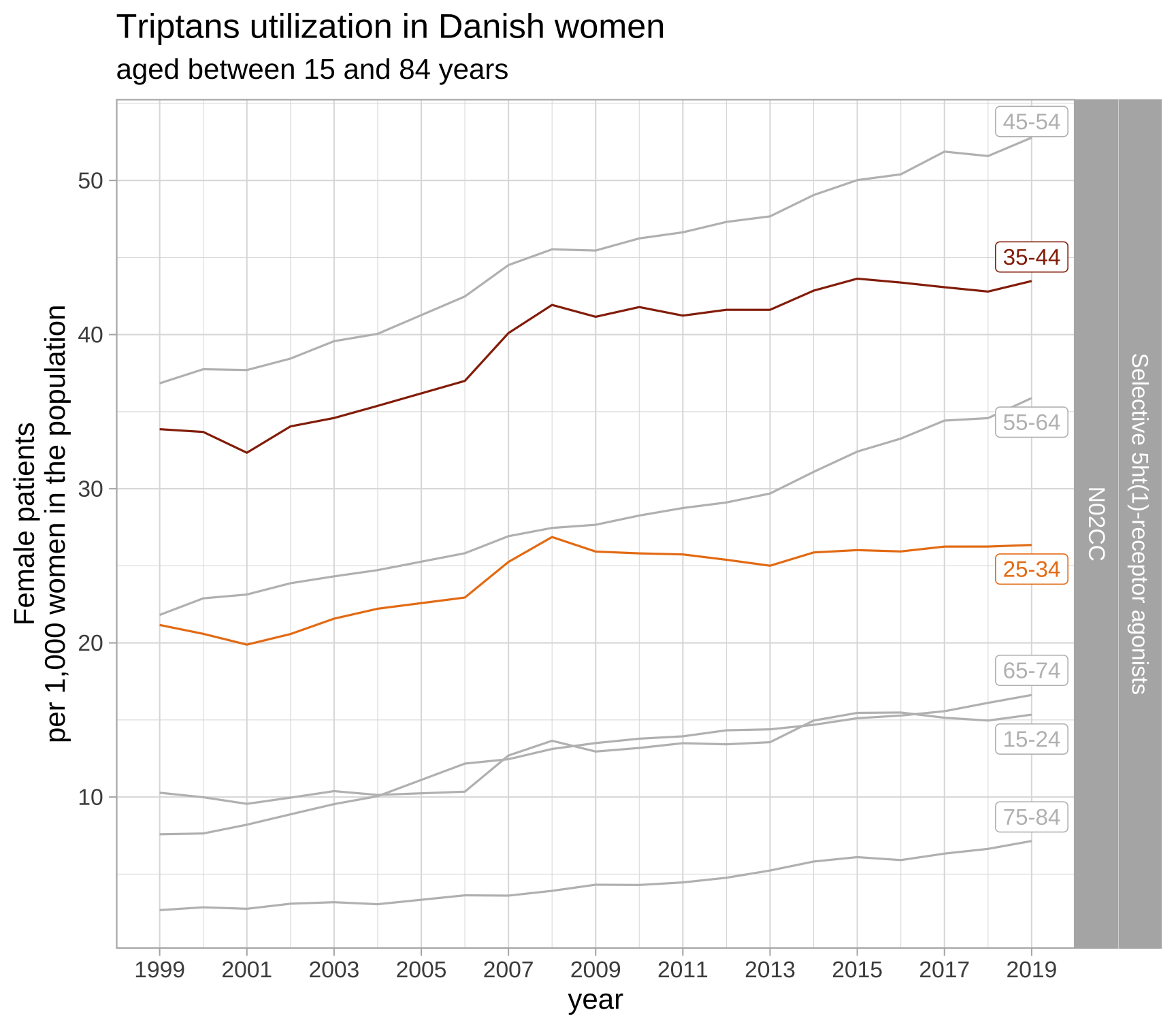
30 / 42
Swedish data
I have Swedish data locally saved, the source can be found here
Keep only the drugs used in migraine, population of women between 18 and 84 on the national level
data_se %<>% filter(gender == "Kvinnor", region == "Riket") %>% filter(str_detect(string = ATC, pattern = all_migraine_drugs))31 / 42
Swedish data is grouped by age categories
data_se %>% distinct(age_group)## # A tibble: 19 x 1## age_group## <chr> ## 1 0-4 ## 2 5-9 ## 3 10-14 ## 4 15-19 ## 5 20-24 ## 6 25-29 ## 7 30-34 ## 8 35-39 ## 9 40-44 ## 10 45-49 ## 11 50-54 ## 12 55-59 ## 13 60-64 ## 14 65-69 ## 15 70-74 ## 16 75-79 ## 17 80-84 ## 18 85+ ## 19 Totalt32 / 42
Categorize age groups according to Danish data
data_se %<>% filter(! age_group %in% c("0-4", "5-9", "10-14", "85+", "Totalt")) %>% # re-group ages as is Danish data mutate( age_cat = case_when( age_group == "15-19" | age_group == "20-24" ~ "15-24", age_group == "25-29" | age_group == "30-34" ~ "25-34", age_group == "35-39" | age_group == "40-44" ~ "35-44", age_group == "45-49" | age_group == "50-54" ~ "45-54", age_group == "55-59" | age_group == "60-64" ~ "55-64", age_group == "65-69" | age_group == "70-74" ~ "65-74", age_group == "75-79" | age_group == "80-84" ~ "75-84", T ~ "other" ) )33 / 42
Compute denominatirs for medication utilization rate
data_se %<>% group_by(ATC, year, age_cat) %>% mutate( numerator = sum(`Antal patienter`), denominator = sum(Befolkning), patients_per_1000_inhabitants = numerator / denominator * 1000 ) %>% filter(row_number() == 1) %>% ungroup() %>% select(year, ATC, gender, age_cat, patients_per_1000_inhabitants) %>% mutate( country = "Sweden" )34 / 42
Add English labels to the ATC codes in Swedish data
data_se %<>% left_join(eng_drug)## Joining, by = "ATC"35 / 42
Check if all medication utilization was available
data_se %>% distinct(ATC, drug) %>% filter(is.na(drug))## # A tibble: 3 x 2## ATC drug ## <chr> <chr>## 1 N02CD01 <NA> ## 2 N02CD03 <NA> ## 3 N02CX07 <NA># fix missing label for N02CD01data_se %<>% mutate( drug = case_when( ATC == "N02CD01" ~ "Erenumab", ATC == "N02CD03" ~ "Galcanezumab", ATC == "N02CX07" ~ "Erenumab", T ~ drug ))36 / 42
Make a plotting function for Swedish data
plot_utilization_se <- function(data, drug_regex, title, max_year){ data %>% filter(! is.na(patients_per_1000_inhabitants)) %>% mutate(label = if_else(year == max_year, as.character(age_cat), NA_character_), value = case_when( age_cat == "25-34" ~ "#EA7F15", age_cat == "35-44" ~ "#962A06", T ~ "gray" )) %>% filter(str_detect(ATC, {{ drug_regex }})) %>% ggplot(aes(x = year, y = patients_per_1000_inhabitants, group = age_cat, color = value)) + geom_line() + facet_grid(rows = vars(drug, ATC), scales = "free", drop = F) + theme_light(base_size = 14) + scale_x_continuous(breaks = c(seq(2006, 2019, 2))) + scale_color_identity() + theme(plot.caption = element_text(hjust = 0), legend.position = "none", panel.spacing = unit(0.8, "cm")) + labs(y = "Female patients\nper 1,000 women in the population", title = paste0(title, " utilization in Swedish women"), subtitle = "aged between 15 and 84 years") + ggrepel::geom_label_repel(aes(label = label), na.rm = TRUE, nudge_x = 3, hjust = 0.5, direction = "y", segment.size = 0.1, segment.colour = "black", show.legend = F)}37 / 42
Set argument lists for the plotting functon and iterate
# no tolfenamiclist_regex_se <- list(regex_triptans, regex_ergots, regex_nsaid, regex_naproxen, regex_erenumab, regex_paracet, regex_salyc_acid_caff, regex_metoclopramide, regex_domperidone, regex_metoprolol, regex_propanolol, regex_topiramate, regex_valproate, regex_flunarizine, regex_amitriptyline, regex_gabapentin, regex_pizotifen, regex_lisinopril, regex_candesartan, regex_botulinum)list_title_se <- list("triptans", "ergots", "NSAIDs", "naproxen", "erenumab", "paracetamol", "salycilic acid and caffeine", "metoclopramide", "domperidone", "metoprolol", "propanolol", "topiramate", "valproate", "flunarizine", "amitriptyline", "gabapentin", "pizotifen", "lisinopril", "candesartan", "botulinum") %>% map_if(. != "NSAIDs", ~ str_to_sentence(.))list_plots_se <- pmap(list(list_regex_se, list_title_se), ~plot_utilization_se(data = data_se, drug_regex = ..1, title = ..2, max_year = 2019)) %>% setNames(., c("triptans", "ergots", "NSAIDs", "naproxen", "erenumab", "paracetamol", "salycilic acid and caffeine", "metoclopramide", "domperidone", "metoprolol", "propanolol", "topiramate", "valproate", "flunarizine", "amitriptyline", "gabapentin", "pizotifen", "lisinopril", "candesartan", "botulinum"))38 / 42
Swedish results
results_se <- data_se %>% filter((age_cat == "25-34" | age_cat == "35-44"), year == "2019", !is.na(patients_per_1000_inhabitants)) %>% select(ATC, drug, age_cat, patients_per_1000_inhabitants, country)39 / 42
Combine Danish and Swedish results
results_se %>% full_join(results_dk) %>% arrange(ATC, age_cat) %>% pivot_wider(names_from = country, values_from = patients_per_1000_inhabitants) %>% slice(1:10) %>% kableExtra::kable(format = "html")## Joining, by = c("ATC", "drug", "age_cat", "patients_per_1000_inhabitants", "country")| ATC | drug | age_cat | Sweden | Denmark |
|---|---|---|---|---|
| A03FA01 | Metoclopramide | 25-34 | 9.1902997 | 9.9674074 |
| A03FA01 | Metoclopramide | 35-44 | 8.4018666 | 7.4055908 |
| A03FA03 | Domperidone | 25-34 | 0.0416631 | 1.6406237 |
| A03FA03 | Domperidone | 35-44 | 0.0689072 | 1.7480274 |
| C07AA05 | Propranolol | 25-34 | 8.1171163 | 4.4959136 |
| C07AA05 | Propranolol | 35-44 | 10.0428186 | 5.2355274 |
| C07AB02 | Metoprolol | 25-34 | 6.2710111 | 3.7127012 |
| C07AB02 | Metoprolol | 35-44 | 12.2911151 | 9.8322977 |
| C09AA03 | Lisinopril | 25-34 | 0.0086199 | 0.2967962 |
| C09AA03 | Lisinopril | 35-44 | 0.0512798 | 0.8212592 |
40 / 42
Combine Danish and Swedish plots
cowplot::plot_grid(list_plots_dk$triptans, list_plots_se$triptans)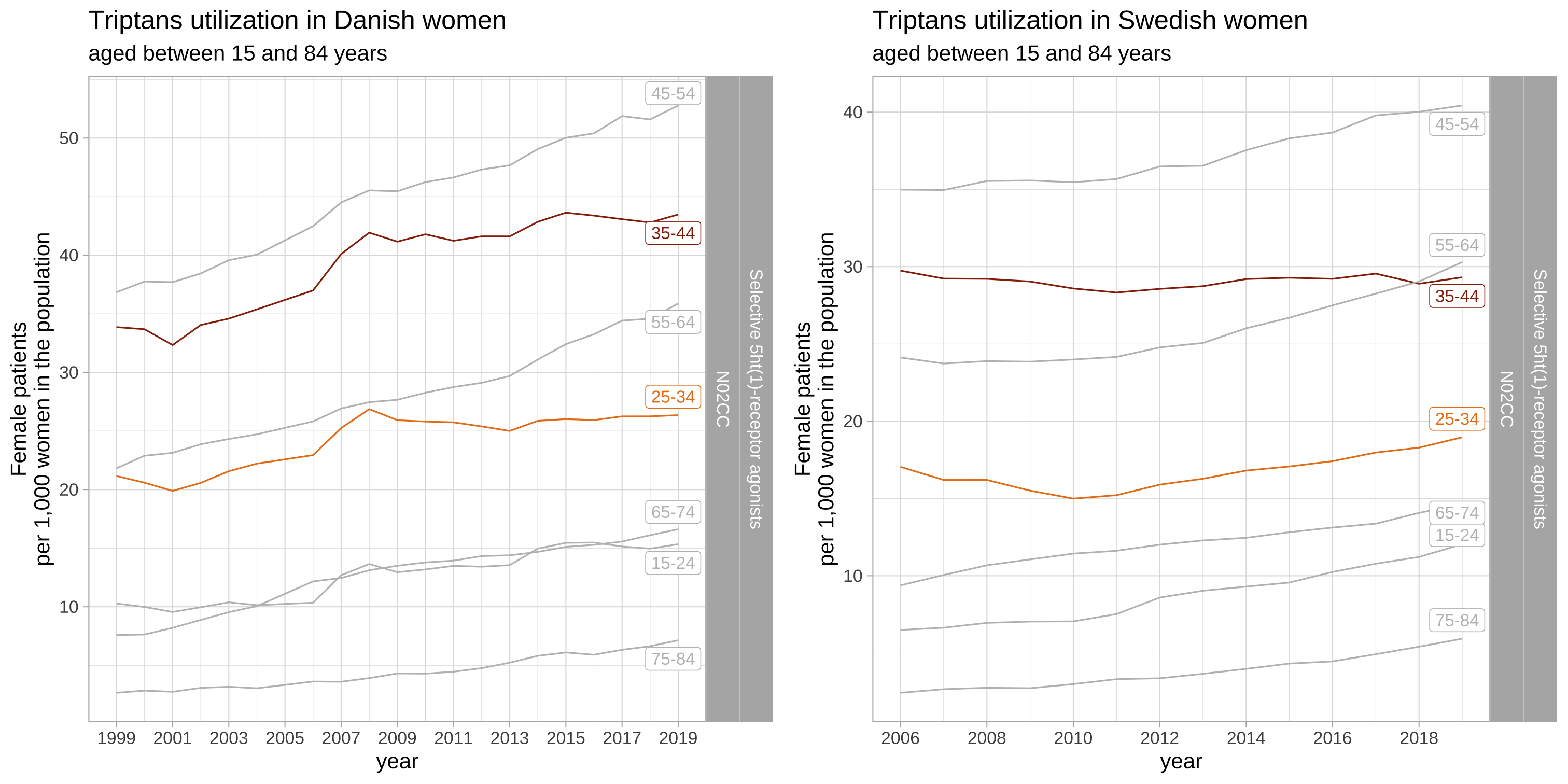
41 / 42
Visit a full blog post
42 / 42